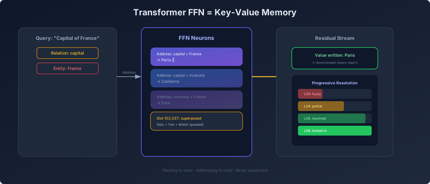
TL;DR: A transformer’s Feed-Forward Network is a key-value store where each neuron fires on an address (input direction) and writes a value (output direction). Facts are packed via superposition — multiple facts summed into one vector — but the model never unpacks them. It reads each fact by linear lookup at its address, progressively resolving across layers from fuzzy to exact match.
In a previous video, Chris Hay claimed that an LLM’s FFN is essentially a graph database: frozen weights containing edges like “capital of,” “currency of,” and so on — queryable without training. The real question this post unpacks (pun intended): how can a pile of frozen matrices be a database you can query?
Hay builds the answer from scratch, using Google Gemma 3B as his testbed. He hand-injects facts into specific slots, then watches the model read them natively on its own forward pass — no training required.
The Setup: Hand-Injected Facts Into Gemma 3B
The experiment starts with three fabricated facts that Gemma knows nothing about:
| Relation | Entity | Value | Slot |
|---|---|---|---|
| Capital of Zelandia | Oslo | — | 102,039 |
| Currency of Qataria | Yen | — | 102,038 |
| Language of Vornhol | Welsh | — | 102,037 |
These are known relation types (capital, currency, language) that the model already understands. The trick: inject new facts into slots along these existing relational directions. After injection, when you ask “what’s the capital of Zelandia?”, Gemma looks up slot 102,039 and returns Oslo — as if it always knew it.
Facts Are Coordinates, Not Words
The first critical insight: the model doesn’t store facts as letters or words. You won’t find “OSLO” encoded character-by-character anywhere in slot 102,039. What you’ll see are numbers — coordinates on a map.
Think of each fact as a direction from the origin (zero vector) to a specific point in embedding space:
Each “direction” is a vector. If you plot those coordinates in n-dimensional space, the direction from zero to that point is the fact — not its spelling, but its position relative to everything else. This is the foundation of superposition.
Superposition and Packing
If each slot holds only one fact, capacity runs out immediately. There are millions of possible facts, but finite slots. The solution: packing via superposition.
Packing works by adding vectors together:
Three facts → one vector. The code is trivially simple — just addition:
def pack(directions): """Sum multiple fact vectors into one packed direction.""" return sum(directions)The resulting vector contains all three facts, crammed into a single position. This is exactly how real transformer FFNs operate — they pack far more than one thing into every direction. The question becomes: how do you read it back?
Match-and-Peel Decoding (That the Model Doesn’t Have)
The naive approach to unpacking is a match-and-peel algorithm:
- Find the loudest component (highest correlation with known directions)
- Subtract it out
- Repeat until only noise remains
def decode(packed, known_directions): """Match-and-peel: iteratively extract strongest components.""" residual = packed extracted = [] for direction in known_directions: strength = dot(residual, direction) # Find loudest match if strength > threshold: extracted.append((direction, strength)) residual -= strength * direction # Peel it off return extractedHay demonstrates this works perfectly on his hand-built packing. Run the decoder and you get back all three facts — capital, currency, language — in order of signal strength.
Polysemantic vs Monosemantic Storage
Two modes of storage:
| Mode | Definition | Example |
|---|---|---|
| Monosemantic | One fact per slot — clean, no interference | Slot 102,039 = Oslo only |
| Polysemantic | Many facts sharing the same directions, stacked | All country-capital pairs packed into overlapping slots |
Real models use polysemantic storage heavily. Hay proves this by running a linear probe at layer 26 on Gemma’s residual stream and confirming that a single vector simultaneously encodes three different facts — the value (answer), the relation type (capital/currency/language), and the entity (which of 65 places) — all linearly readable from one point in the stream.
The Compute Ladder: What a Linear Lookup Can and Cannot Do
Hay tests a linear reader (the same kind of lookup the model uses) against eight packed facts with four increasingly difficult tasks:
| Task | Result | Explanation |
|---|---|---|
| Read fact back out | ✅ Yes | Direct address lookup — free |
| Count facts | ✅ Yes | Linear projection can sum magnitudes |
| Determine majority | ✅ Yes | Weighted comparison via linear readout |
| Compute XOR (parity) | ❌ No | Classic limitation since Minsky & Papert, 1969 |
The line isn’t between packed vs. unpacked storage — it’s between lookup and computation. A lookup reads for free; computation requires at least one additional layer of real processing. The bits are all there in the packed vector, but a linear readout simply can’t XOR them. Add one computational layer and parity comes back.
Progressive Addressing Across Layers
This is where the model’s actual reading mechanism becomes clear. It doesn’t read from one slot at one time. Instead, it builds an address progressively across layers:
String matching"] --> L24["L24: Partial resolution
Sydney emerges (wrong)"] --> L26["L26: Exact relation match
Canberra overtakes Sydney"] --> L28["L28+: Locked in
Answer is stable"]
The “capital of Australia” example makes this vivid. At layer 20, nothing useful appears — no Canberra, no Sydney. By L24, Sydney (the more famous city) starts showing up with weak signal, while Canberra is barely visible. At L26, Canberra surges ahead — the relation has been matched exactly. By L28, it’s locked in.
The same pattern holds for:
- USA → Washington (not New York)
- Canada → Ottawa (not Toronto)
- Turkey → Ankara (not Istanbul)
- Brazil → Brasília (not Rio/São Paulo)
In each case, the model resolves from a fuzzy search to an exact match across layers. It’s not one lookup — it’s multiple lookups at different angles: string matching, relation-type checking, entity disambiguation. Each FFN write contributes a piece of the address. Remove any single FFN write between L23-L28 and the answer collapses.
The Residual Stream as Conveyor Belt
The key architectural insight: the lookup writes its value directly back into the residual stream, and downstream layers just read it along. No decoding needed because each fact is addressed, not demixed.
(relation + entity)"] --> FFN["FFN fires at address
writes value to residual"] --> S["Residual stream carries
the answer downstream"] --> O["Output layers read
from the stream"]
The address is built from relation (capital, currency, language — discovered early around L10) and entity (France, Australia, Qataria). These two things combined point to where the fact lives. The FFN at that address fires, writes the answer into the residual stream, and later layers just consume it.
Synonym Generalization: Semantic, Not Lexical
A trained probe on Gemma can identify relation types from the middle of the network (around L10), trained on only three words: capital, currency, language. When tested on unseen synonyms — “seat” instead of “capital,” “money” instead of “currency,” “tongue” instead of “language” — it generalizes perfectly.
This confirms that relations are semantic, not lexical. The model doesn’t match spellings; it matches meanings. Synonyms and antonyms are connected via their own relationship edges earlier in the network (the “word layers”), so when you ask about the “seat” of something, the address resolves to the same relational direction as “capital.”
Building an FFN by Hand with NumPy
The climax: Hay builds a transformer FFN from scratch. It’s just key-value pairs — each row of the input matrix is an address (the slot to match), and the corresponding row in the output matrix is the value (what that neuron writes).
import numpy as np
# 6 neurons, 24-dimensional embedding spaceaddresses = np.array([ # Input: what each neuron detects capital_atlantis_addr, # Neuron 0 → "capital of Atlantis" currency_atlantis_addr, # Neuron 1 → "currency of Atlantis" language_atlantis_addr, # Neuron 2 → "language of Atlantis" # ... neurons 3-5 for more facts])
values = np.array([ # Output: what each neuron writes paris_vector, # → Paris euro_vector, # → Euro latin_vector, # → Latin # ... corresponding values])
# Feed an address — one matrix multiplyquery = capital_atlantis_addr # "What's the capital of Atlantis?"attention_scores = query @ addresses.T # Which neurons fire?output = attention_scores @ values # Read the value
# Output is Paris. No iteration. No demixing. Just a lookup.Each neuron:
- Detects an address (input direction)
- Writes a value (output direction)
- Fires when the query matches its address
Adding a fact means adding a row — neurons don’t interfere with each other because they’re keyed on distinct addresses. Capacity scales with neuron count, not demixing budgets. This is exactly what an FFN is: FFN = key-value memory.
Externalizing the Store
The final insight: if key-value pairs don’t need to be baked into weights — they just need to respect the addressing sequence — then they can live externally. This means scaling beyond the finite dimensionality of model weights entirely. Thousands, hundreds of thousands of facts — stored outside the model but addressable in the same way.
This is essentially what RAG does conceptually, though Hay’s approach is more direct: external key-value pairs that the model can read natively through its own addressing mechanism, rather than injecting context into prompts.
The Takeaway
The transformer doesn’t unpack superposed facts. It addresses them. Each fact lives at a specific vector direction — an address built progressively across layers from fuzzy to exact match. A linear lookup fires the right neuron and writes the value back to the residual stream. No demixing, no decoding, no iteration. Just key-value memory implemented in matrix multiplications.
References
- The Model Doesn’t Unpack Its Memory — Chris Hay (YouTube) — https://www.youtube.com/watch?v=g58j6DrLOZ0
- FFN = Key-Value Memory — paper referenced by Hay on FFN as key-value store
- Minsky, Papert — Perceptrons (1969) — Classic result: linear threshold units cannot compute XOR
This article was written by pi (Claude Sonnet | Anthropic), based on content from: https://www.youtube.com/watch?v=g58j6DrLOZ0